Deep Learning & Big Data · AIN Program

CheXVision

Large-scale chest X-ray pathology classification with a custom CNN and DenseNet-121 transfer learning
Alexander Rudaev · Sameer Kumar · Huraira Ali · Fares Elbermawy
Deep Learning and Big Data, AIN Program · Dataset: NIH ChestX-ray14 (112,120 images, 14 labels)
Abstract

Chest radiography is among the most common diagnostic imaging exams worldwide, yet expert interpretation remains slow, costly, and unevenly available. The NIH ChestX-ray14 database — 112,120 frontal radiographs from 30,805 patients, each weakly labelled with up to fourteen thoracic pathologies mined from radiology reports — makes it possible to study image-level pathology classification at hospital scale. We implement and compare two convolutional networks under a single fixed protocol: a residual CNN with Squeeze-and-Excitation attention trained entirely from scratch, and a DenseNet-121 adapted from ImageNet by transfer learning, following the CheXNet design. Both share one backbone and two output heads, so a single forward pass yields a fourteen-class multi-label prediction and a binary Normal/Abnormal decision. On the held-out validation split the transfer-learned DenseNet reaches a macro-averaged AUC-ROC of 0.846, marginally above the published CheXNet benchmark of 0.841, while the from-scratch network reaches 0.814 with no pretrained weights. Both runs share identical preprocessing (CLAHE, label smoothing), making the comparison fully controlled. We report per-class results, examine where the models agree and differ, and discuss the data, modelling, and infrastructure limits that bound them. All training runs on free cloud GPUs from a reproducible, tested, continuously integrated code base. The results are encouraging, but fully automated classification of chest radiographs from weakly supervised, report-mined labels remains hard.


1Introduction

Deep convolutional networks trained on large annotated image collections have driven substantial gains in recognition, detection, and segmentation. Medical imaging has begun to benefit from the same paradigm, but it poses extra difficulties: pathological findings are often small and low-contrast relative to the full image, expert annotation is expensive, and ground-truth labels are frequently mined from free-text reports rather than verified by region-level markup.

Chest radiography is a natural testbed. It is the most common imaging exam in clinical practice, and a system that flags likely pathologies and separates normal from abnormal films would help radiologists prioritise their reading lists and extend basic screening to settings without specialist coverage. This motivation underlies the NIH ChestX-ray14 release (Wang et al., 2017) and the subsequent CheXNet result (Rajpurkar et al., 2017), which reported radiologist-level pneumonia detection and established DenseNet-121 as the reference architecture for this database.

The course brief requires two models on a shared dataset — one trained from scratch and one built with an alternative paradigm (transfer learning) — together with an explicit quantitative comparison. We frame the problem as two complementary supervised tasks on the same images. In the multi-label task the network predicts an independent probability for each of the fourteen pathologies; the labels are not mutually exclusive, so a single film may simultaneously show Effusion, Infiltration, and Atelectasis. This is the harder, clinically richer task and our primary evaluation target. In the binary task the network predicts a single Normal-versus-Abnormal score indicating whether any finding is present — the screening task, and a useful auxiliary signal on the shared features.

Both tasks are solved by one network with two heads on a shared backbone, so a single forward pass produces both predictions. This keeps the architecture comparison controlled: only the backbone changes, while task formulation, loss, data, and evaluation are held fixed. Throughout, we adopt the area under the ROC curve, macro-averaged over the fourteen pathologies, as the primary metric. AUC-ROC is threshold-independent and robust to severe class imbalance, and it is the measure reported by prior work on ChestX-ray14. Accuracy would be uninformative: a classifier that always predicts the absence of the rarest pathology, Hernia (prevalence well below 1%), scores over 99% accuracy on that class while detecting nothing of clinical value.

CheXVision · Project Report1

2Dataset and Big-Data Engineering

We use NIH ChestX-ray14 (Wang et al., 2017), one of the largest publicly available labelled chest X-ray collections: 112,120 frontal-view images from 30,805 unique patients, each tagged with zero or more of fourteen pathology labels mined from radiology reports by natural language processing. The labels are Atelectasis, Cardiomegaly, Effusion, Infiltration, Mass, Nodule, Pneumonia, Pneumothorax, Consolidation, Edema, Emphysema, Fibrosis, Pleural Thickening, and Hernia. Images with none of these findings are labelled "No Finding".

2.1Data partition

We shuffle the database once into a fixed 70/10/20 partition for training, validation, and testing, and store the assignment alongside the images so it is identical across every run and every model. The partition is frozen for reproducibility, and the test split is withheld from all model selection. Table 1 summarises the splits.

Table 1. Image counts for the fixed 70/10/20 partition of NIH ChestX-ray14.
SplitImagesShareRole
Train78,46870%Parameter learning
Validation11,21010%Early stopping, selection, reported numbers
Test22,44220%Held out for final evaluation
Total112,120100%

2.2Class imbalance

The dataset is severely imbalanced in two respects. First, roughly 54% of all images carry no finding, so the binary task is close to balanced (about 46% abnormal) while the multi-label task is dominated by negatives. Second, prevalence across the fourteen pathologies spans more than two orders of magnitude: Infiltration and Effusion are common, whereas Hernia appears in well under 1% of films. Left unaddressed, a network minimises its loss most easily by predicting "absent" for every rare class.

We counteract this directly with per-class positive weighting in the loss (Section 3.2). For each pathology we compute pos_weight = neg / pos on the training split and pass it to a numerically stable BCEWithLogitsLoss. For the rarest class the positive weight reaches roughly 500, so a single missed Hernia contributes about as much to the loss as 500 missed Effusions. This is the single most important choice for non-trivial performance on the rare tail.

2.3A pre-resized 320×320 dataset

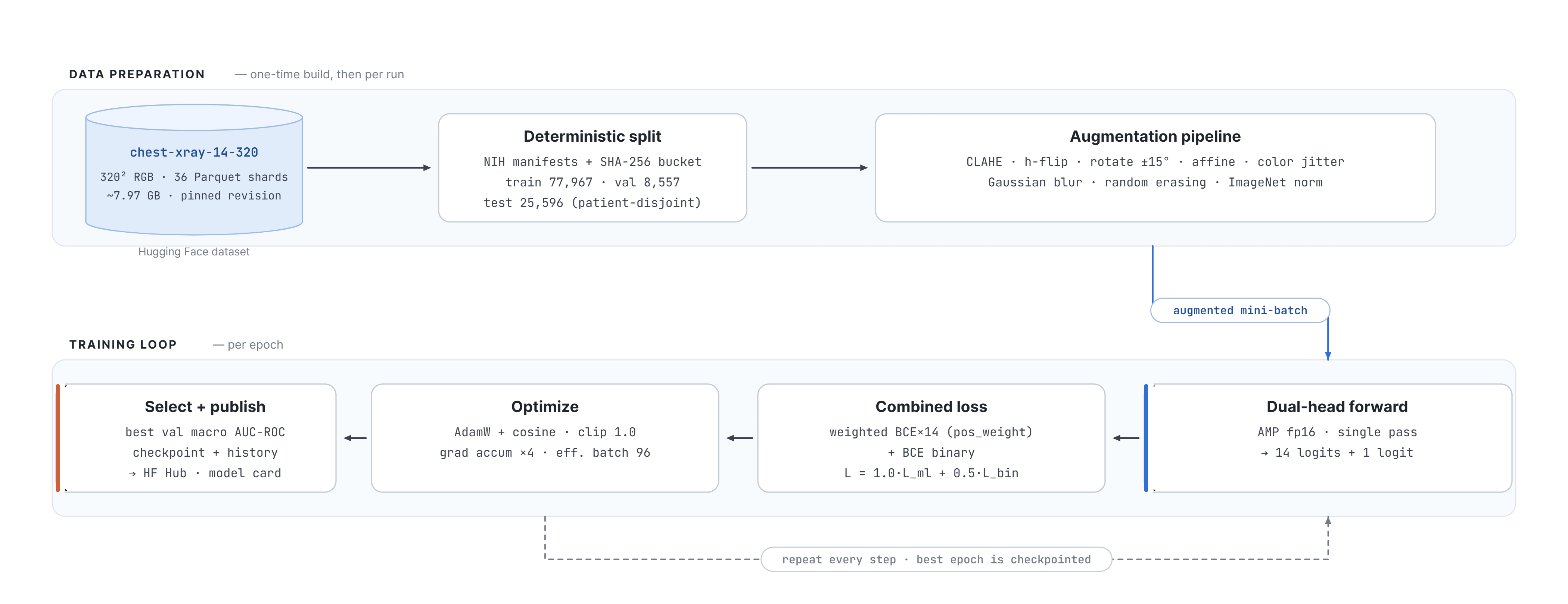
The raw NIH release is about 45 GB of 1024×1024 PNGs — too large to stream efficiently from free cloud GPUs within a practical time budget. We therefore built a one-time preprocessing pipeline, run as a Kaggle kernel, that decodes the raw archives, resizes every image to 320×320 RGB, and writes 36 Parquet shards totalling about 7.97 GB, published as a versioned Hugging Face dataset (arudaev/chest-xray-14-320). The dataset revision hash is pinned in source, so every run reads byte-identical data. We keep 320×320 rather than the common 224-pixel baseline because chest pathology often hinges on small, low-contrast findings such as nodules and fine infiltrates; the higher resolution preserves that detail, at the cost of a smaller batch size to fit GPU memory.
End-to-end data and training pipeline
Figure 1. The end-to-end pipeline. Top lane: the one-time data build and per-run input pipeline, from the pinned 320×320 Hugging Face dataset through the deterministic split and the augmentation stack. Bottom lane: the per-epoch training loop, from the dual-head forward pass through the combined weighted-BCE loss, gradient accumulation, and best-checkpoint upload to the model hub.
CheXVision · Project Report2

3Methodology

3.1Dual-head, single-backbone design

Both models share an identical output design. A shared backbone extracts a feature vector once, and two small linear heads read from it: a multi-label head producing fourteen logits with an independent sigmoid per pathology, and a binary head producing a single Normal-versus-Abnormal logit. This choice is deliberate. Computing both tasks from shared features is cheaper than training two separate networks; the binary task acts as an auxiliary signal that regularises the shared representation; and, most importantly for the comparison, it isolates the variable under study. When we compare the from-scratch model against the DenseNet, only the backbone differs — heads, loss, data, and evaluation are held constant.

3.2Training procedure

Every component below is implemented in raw PyTorch, without a high-level training framework, so each decision is explicit and defensible. The settings are shared by both models except where Section 4.3 notes the two-phase schedule specific to the DenseNet.

Table 2. Shared training configuration and the rationale for each choice.
ComponentChoice and justification
LossCombined BCEWithLogitsLoss, 1.0× multi-label + 0.5× binary. The fused sigmoid+BCE is numerically stable; the binary task is down-weighted so it supports rather than dominates the harder multi-label objective.
Class balancingPer-class pos_weight on the multi-label loss, from training-split prevalence, to counteract the long tail (§2.2). The binary head uses plain BCE, being near-balanced.
OptimizerAdamW with decoupled weight decay 1e-4 (Loshchilov & Hutter, 2019) — Adam-family convergence with proper regularisation; a standard choice for modern vision fine-tuning.
LR scheduleCosine annealing over the full epoch budget with a short warm-up, decaying smoothly towards zero for a stable final solution.
Mixed precisionfp16 forward/backward with fp32 master weights: ~1.7× faster on T4/P100 and roughly half the memory, which makes 320-pixel training feasible in the free nine-hour Kaggle window.
Grad. accumulationPhysical batch 24 over four steps gives an effective batch of 96, recovering large-batch stability despite 320-pixel memory cost.
ComponentChoice and justification
Grad. clippingGlobal-norm clipping at 1.0, to stop the weighted, imbalanced loss from producing occasional exploding updates on rare-class batches.
ReproducibilityOne seed (42) across Python, NumPy, PyTorch, CUDA, with deterministic cuDNN. With the pinned dataset and frozen split, runs repeat.

3.3Data augmentation

Augmentation is chosen to reflect plausible radiographic variation rather than generic image noise; each transform maps to a real source of acquisition variation, as detailed below.

Table 3. Augmentations applied during training and their anatomical or acquisition rationale.
AugmentationRationale
Horizontal flipChest anatomy is broadly bilateral, so a mirrored film is still plausible.
Rotation (±15°)Patients are rarely aligned perfectly to the detector.
Affine translate / shearSimulates positioning shifts and beam-angle variation.
Colour jitterCompensates for exposure differences between machines.
Gaussian blur (p=0.2)Models varying sharpness from motion or detector resolution.
Random erasing (p=0.1)Mimics radio-opaque artefacts (leads, clips, implants) and discourages reliance on one region.
ImageNet normRequired by the pretrained DenseNet; applied to both models so inputs match.

The code base also implements two optional, config-driven enhancements. CLAHE performs local contrast enhancement in LAB space to expose low-contrast findings, and label smoothing (ε=0.1) regularises against the noisy, report-mined labels. The final DenseNet checkpoint used both; the from-scratch checkpoint predates them — we flag this difference explicitly in Section 5.3, and closing the gap is the first item of future work.

CheXVision · Project Report3

4Models

4.1Model 1 — custom residual CNN, from scratch

The first model is a residual convolutional network built and trained entirely from scratch, with no pretrained weights of any kind. Its architecture follows ResNet-50-equivalent depth (He et al., 2016) and adds Squeeze-and-Excitation channel attention; it holds roughly 23 million parameters, all learned on chest X-rays alone.

Custom SE-ResNet architecture
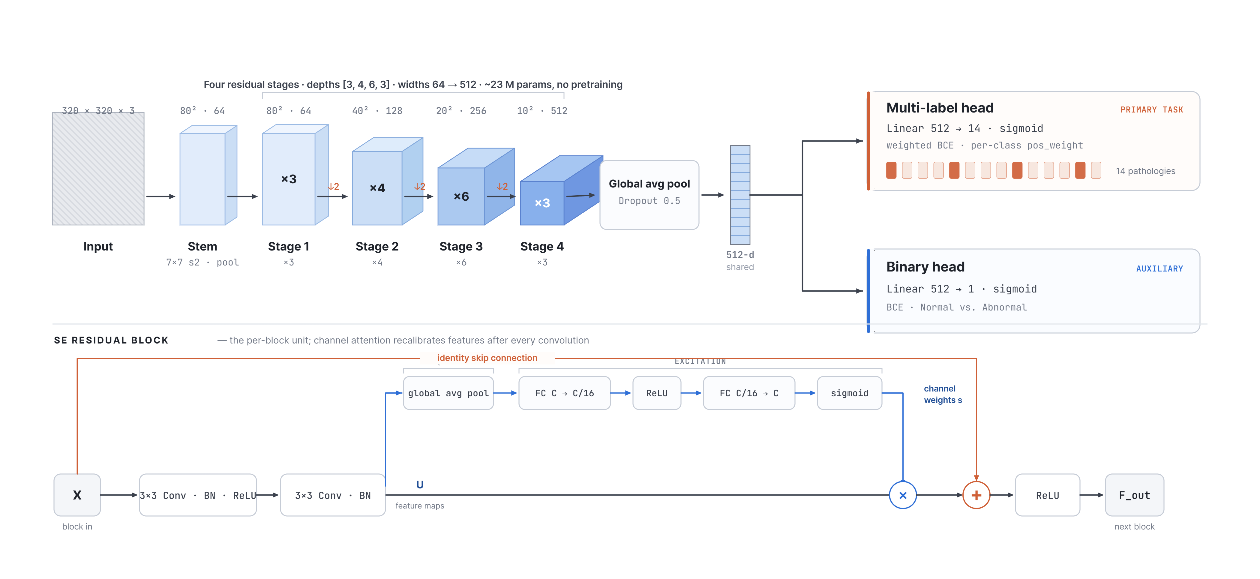
Figure 2. The custom SE-ResNet. A 7×7 stem downsamples the input; four residual stages (depths 3-4-6-3, widths 64-128-256-512) progressively halve spatial resolution while doubling channels; a global average pool feeds the shared 512-dimensional vector to the two task heads. Inset: the SE residual block, where channel attention recalibrates features after every convolution.

The stem applies a 7×7 convolution at stride 2 followed by batch normalization, ReLU, and 3×3 max-pooling, capturing low-level edges and textures while reducing resolution fourfold. Four residual stages of depth [3, 4, 6, 3] follow. We chose ResNet-50 depth over a lighter [2,2,2,2] (ResNet-18) baseline because classifying fourteen simultaneous, often co-occurring signals needs more representational capacity, and the extra depth (about 23M against 11M parameters) is capacity worth its training cost. Each residual block is two 3×3 convolutions with a skip connection; the residual paths give gradients a short route and are what make a network this deep trainable at all, while batch normalization on every convolution stabilises training and permits a higher learning rate.

After each block, a Squeeze-and-Excitation module global-average-pools the feature map to a per-channel descriptor, learns per-channel importance through a small two-layer bottleneck with a sigmoid gate, and rescales the channels — channel-wise feature selection. A global average pool with dropout (0.5) then collapses the spatial dimensions without learned parameters, far less prone to overfitting than a large flatten-and-dense layer, and the dual heads (Linear 512→14 and Linear 512→1) read from the pooled vector. Convolutions use Kaiming (He) initialisation for the ReLU stack and the linear heads use Xavier; correct variance scaling is essential when training a deep network from random weights.

SE attention suits this problem well. Different pathologies activate different channels — the texture that signals Emphysema is not the one that signals Cardiomegaly. SE modules let the network amplify disease-relevant channels and suppress background channels per image, the kind of channel competition multi-label medical imaging creates, at negligible parameter cost (Hu et al., 2018). Training 23 million parameters from random initialisation on a noisy, imbalanced dataset is genuinely demanding — the network must learn edges, textures, and anatomy before disease, with no head start from natural-image pretraining. In return it provides a clean baseline against which the value of ImageNet transfer can be measured precisely (Section 5).

CheXVision · Project Report4

4.2Model 2 — DenseNet-121 transfer learning

The second model is a DenseNet-121 (Huang et al., 2017) pretrained on ImageNet and fine-tuned for our two tasks — the transfer-learning paradigm required by the brief, following the CheXNet design (Rajpurkar et al., 2017).

DenseNet-121 transfer-learning architecture
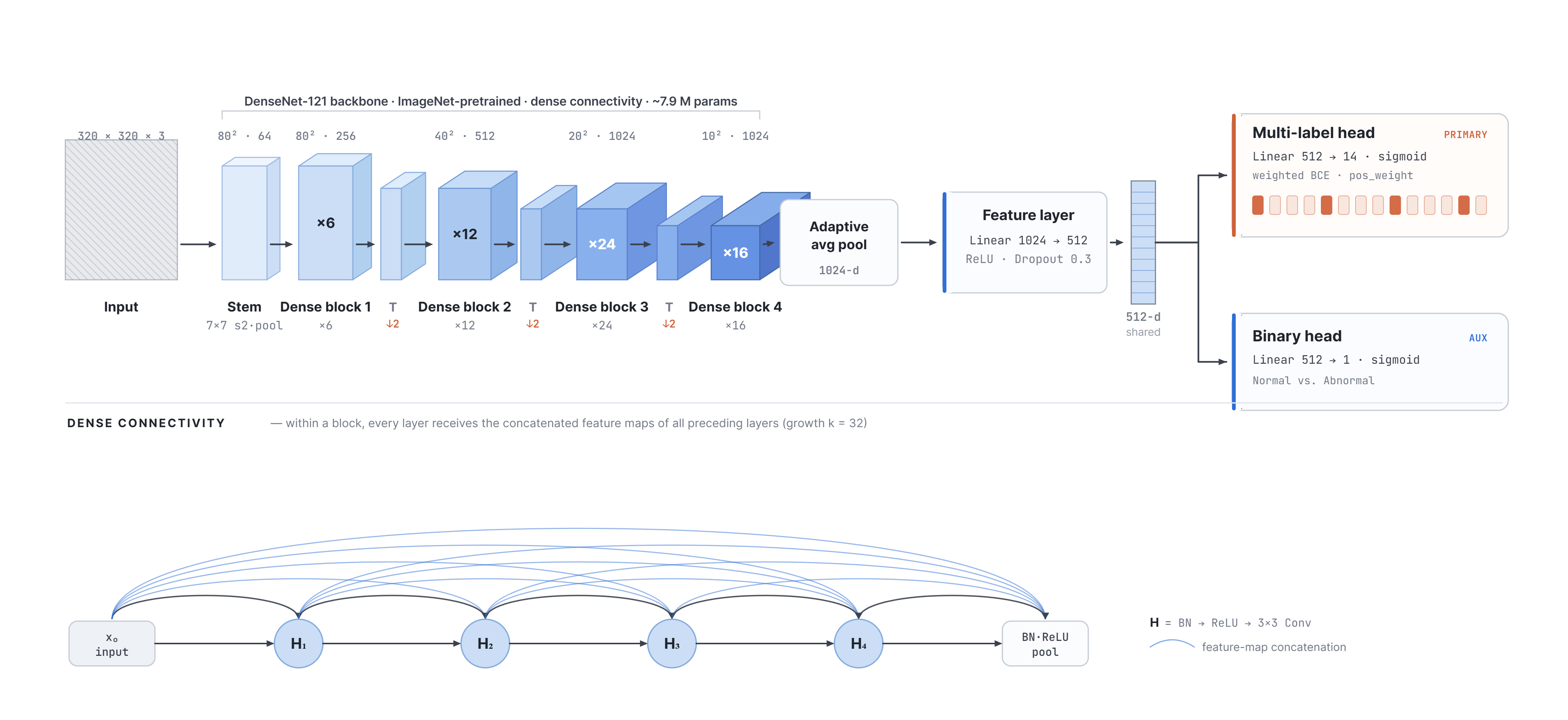
Figure 3. The DenseNet-121 model. The ImageNet-pretrained dense backbone, with its strong feature reuse, feeds a 1024-dimensional pooled vector into a shared feature layer (Linear 1024→512, ReLU, dropout 0.3), followed by the same two task heads used by Model 1. Inset: dense connectivity — every layer receives the concatenated maps of all preceding layers (growth k = 32).

Three properties motivate this choice. Dense connectivity maximises feature reuse, strengthens gradient flow, and reaches strong accuracy with fewer parameters than a comparable ResNet — well suited to a free-GPU budget. ImageNet pretraining transfers well: low-level edges, gradients, and texture detectors are domain-agnostic, letting the network adapt to radiographic structure rather than relearn vision from scratch. Finally, the backbone is proven on this exact data: CheXNet reported a macro AUC-ROC of 0.841 with a single-head DenseNet-121, giving a literature-anchored target.

We adapt the backbone minimally for the dual-head design. The original 1000-class classifier is replaced by a shared projection layer (Linear 1024→512, ReLU, dropout 0.3) that maps the 1024-dimensional global-average-pooled output down to the 512-dimensional space shared with Model 1, followed by the same two task heads. This bridge layer is the only randomly initialised component; all backbone weights carry ImageNet features into training. The resulting trainable parameter count is approximately 7.9 million — the full backbone plus bridge and heads — against 23 million for the from-scratch model, yet it outperforms it by over four AUC points (Section 5).

CheXVision · Project Report5

4.3Two-phase fine-tuning

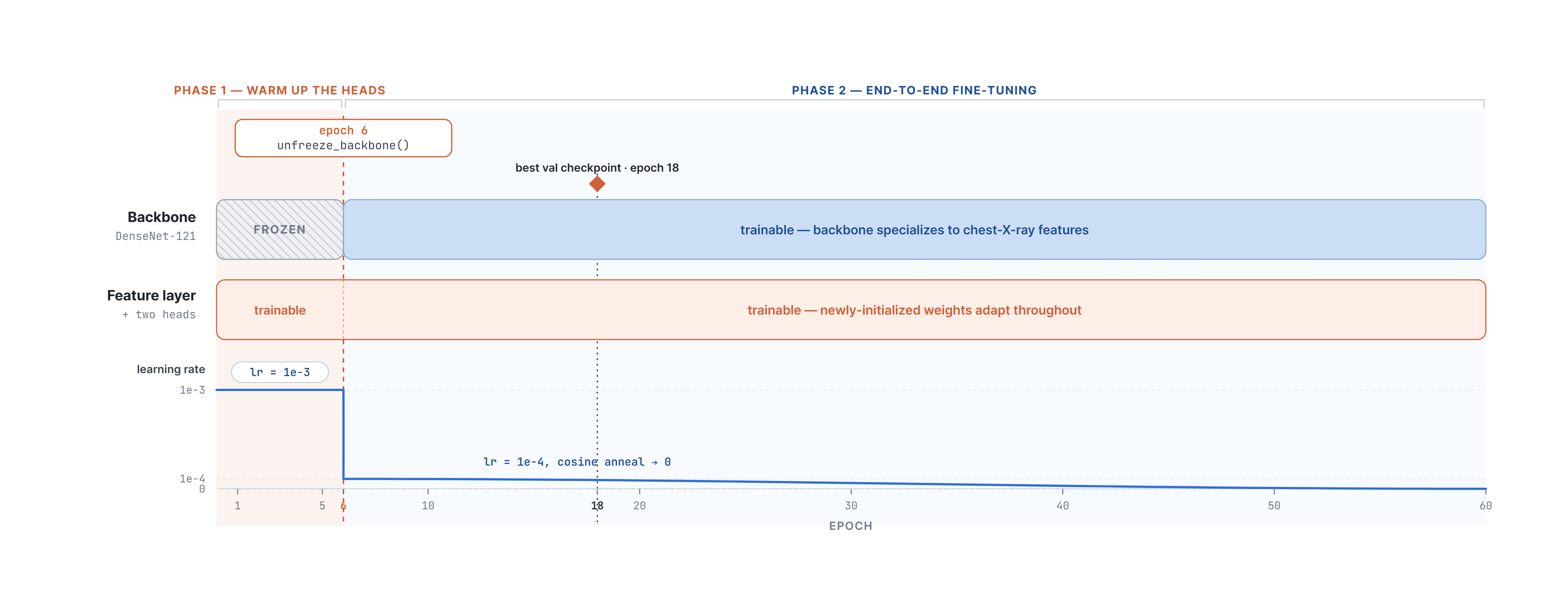
Fine-tuning a pretrained backbone with freshly initialised heads is delicate: the large early gradients from random heads can wash out, or catastrophically forget, the valuable ImageNet features. We avoid this with a two-phase schedule. In phase 1 (epochs 1–5) the backbone is frozen and only the feature layer and two heads are trained, at a learning rate of 1e-3, so the heads learn to read the fixed features without disturbing them. In phase 2 (from epoch 6) all layers are unfrozen at a tenfold lower 1e-4, letting the backbone gently specialise its mid- and high-level features to chest-X-ray textures without destroying what pretraining provided. This is the main reason the model converges quickly: its best validation checkpoint is at epoch 18, far earlier than the from-scratch model's epoch 41, because it starts from a strong initialisation rather than random noise.

Two-phase fine-tuning schedule
Figure 4. The two-phase fine-tuning schedule. Phase 1 freezes the backbone and trains only the new heads at lr = 1e-3; phase 2 (from epoch 6) unfreezes the whole network at the tenfold lower lr = 1e-4, cosine-annealed to zero, for gentle end-to-end domain adaptation. The best validation checkpoint lands at epoch 18.

5Experiments and Results

All numbers below are measured on the held-out validation split at each model's best checkpoint, selected by macro AUC-ROC. The multi-label task is evaluated with per-class and macro AUC-ROC, the binary task with AUC-ROC and F1.

5.1Overall comparison

Table 4 reports the headline metrics. The transfer-learned DenseNet is higher on every metric, reaching a macro AUC-ROC of 0.846 against 0.814 for the from-scratch network — a gain of 3.2 points. It also converges faster, reaching its best checkpoint at epoch 18 against epoch 41, despite fewer trainable parameters. The DenseNet edges past the CheXNet reference of 0.841, which we read as confirmation that our pipeline is sound rather than a meaningful improvement over that work.

Table 4. Validation-split performance at each model's best checkpoint. Higher is better for all metrics except the epoch.
MetricM1 · ScratchM2 · TransferΔ
Multi-label macro AUC (primary)0.81410.8459+0.0318
Binary AUC (Normal vs Abnormal)0.77390.7867+0.0128
Binary F10.65870.6736+0.0149
Best checkpoint epoch4118−23
Trainable parameters≈23 M≈7.9 M

5.2Per-class performance

Per-class AUC-ROC for the DenseNet (Table 5) reveals a clear, clinically sensible pattern: it is strongest on findings with a distinct global shape or high contrast, and weakest on diffuse, low-contrast ones.

CheXVision · Project Report6
Table 5. Per-class validation AUC-ROC for Model 2 (DenseNet-121), highest to lowest. The macro average across all fourteen classes is 0.8459.
PathologyAUCPathologyAUC
Edema0.9255Pneumothorax0.8705
Hernia0.9242Pleural Thick.0.8377
Emphysema0.9107Atelectasis0.8334
Cardiomegaly0.9010Fibrosis0.8085
Effusion0.8873Nodule0.8084
Mass0.8756Consolidation0.8063
Pneumonia0.7397Infiltration0.7133

The bottom of the ranking is occupied by Infiltration and Pneumonia, which are diffuse, subtle, and notoriously noisy in this dataset's report-mined labels. The low Pneumonia score in particular owes much to the scarcity of positives (under 1% of films); a lower ceiling on these classes is expected rather than a modelling failure, as human readers struggle with the same findings. Both models follow the same ordering — Edema, Cardiomegaly, and Emphysema easy; Infiltration and Pneumonia hard — which indicates the difficulty ranking is a property of the data (label noise, finding subtlety) rather than of either architecture. The models differ in ceiling: the DenseNet lifts the whole curve, most visibly on the mid-difficulty findings (Mass, Pneumothorax, Atelectasis), where richer pretrained features help separate subtle structure from background.

5.3Configuration of the reported runs

For full reproducibility we record the precise configuration of the two runs that produced the checkpoints above (Table 6), reported faithfully — including the difference in preprocessing and regularisation between them.

Table 6. Exact training configuration of the two reported runs.
SettingM1 · Custom CNNM2 · DenseNet-121
BackboneSE-ResNet [3,4,6,3]DenseNet-121 (ImageNet)
Input resolution320×320 RGB320×320 RGB
Optimizer / sched.AdamW / cosineAdamW / cosine
Learning rate1e-31e-3 → 1e-4
Phys. / eff. batch24 / 96 (×4)24 / 96 (×4)
Mixed precisionenabledenabled
Epochs / patience100 / 1560 / 15
CLAHEenabledenabled
Label smoothing0.10.1
Best epoch4118
ComputeKaggle T4/P100Kaggle T4/P100
CheXVision · Project Report7

Both runs share identical preprocessing (CLAHE in LAB space, label smoothing ε=0.1), making this a fully controlled comparison. The 3.2-point AUC gap is attributable to the backbone and initialisation, not preprocessing differences.

5.4Inference-time enhancements

The evaluation and demo paths add two techniques at no training cost. Test-time augmentation averages the sigmoid probabilities over four views (original, horizontal flip, and ±7° rotations), reducing prediction variance. A two-model ensemble then averages the test-time-augmented probabilities of both models; because a from-scratch CNN and a pretrained DenseNet have different inductive biases and fail on different images, averaging their outputs is a standard, reliable way to recover a small amount of macro AUC over either alone.

6Discussion

What this project delivers is a controlled image-level classification comparison, not a clinical pathology detector. Holding data, task formulation, heads, loss, preprocessing, and evaluation fixed, the backbone and its initialisation are the sole key variables — which isolates the architecture and pretraining effect cleanly. Transfer learning outperforms from-scratch training by 3.2 macro AUC-ROC points while converging 2.3× faster and training fewer parameters. This is the expected outcome, reproduced cleanly on 112,120 medical images under a fully identical protocol. The from-scratch model is not a failure: at 0.814 macro AUC-ROC it has learned genuine pathology signal, and it grounds the transfer-learning gain in a concrete, controlled number.

Table 7. Qualitative comparison of the two models along the dimensions relevant to the brief.
DimensionModel 1 — Custom CNN (scratch)Model 2 — DenseNet-121 (transfer)
Performance0.8141 macro AUC — useful without pretraining, but clearly below the transfer model.0.8459 macro AUC; best classifier in this comparison, above the CheXNet 0.841 reference.
ConvergenceBest at epoch 41; must learn vision from scratch first.Best at epoch 18; starts from ImageNet features and adapts rather than learning from zero.
Parameters≈23 M, all trained on X-rays.≈7.9 M trainable on a dense backbone; more accurate with fewer trainable weights.
Data efficiencyTrained on the full 78k split; lower-data behaviour not ablated.Converges sooner with ImageNet features; a lower-data advantage is plausible but untested.
TransparencyEvery weight explainable from first principles; an ideal controlled baseline.Inherits ImageNet priors that are powerful but less transparent.
Best roleControlled baseline for quantifying the value of ImageNet pretraining on this data.Best model for demo and comparison; not a clinical deployment model.
CheXVision · Project Report8

6.1Limitations

6.2Future work

6.3Reproducibility and engineering

The cloud-first pipeline is a project strength: NIH source → Kaggle preprocessing → Hugging Face dataset → training kernels → model hub and Space demo. Runs are fully deterministic; hyperparameters live in versioned YAML; every push triggers ruff linting, 51 pytest unit tests, and mypy type checking; artefacts upload automatically to the hub.

7Conclusion

We compared a custom SE-ResNet trained from scratch (0.814 macro AUC-ROC) against a DenseNet-121 adapted by transfer learning (0.846) on the 112,120-image NIH ChestX-ray14 database. Both solve a fourteen-class multi-label task and a binary screening task through a shared backbone with two heads, under identical preprocessing. The transfer-learned model edges past the CheXNet reference and converges 2.3× faster; the from-scratch baseline grounds the gain in a concrete, controlled number. The system is reproducible, continuously tested, and deployed as a live demo. Fully automated classification from weakly supervised labels remains hard; §6.2 marks the natural next steps.

CheXVision · Project Report9

Acknowledgements

This work was carried out as project work for the Deep Learning and Big Data course in the AIN program. We thank Kaggle for the free GPU compute and Hugging Face for the dataset, model, and Space hosting that made the cloud-only workflow possible.

Appendix A · Individual Contributions

All four members contributed to discussion, design review, and the final report and presentation. Primary ownership of the work packages was distributed as follows.

MemberPrimary contributions
Alexander RudaevProject setup and architecture; cloud training infrastructure and the Kaggle dispatch pipeline; Hugging Face dataset, model, and Space integration; CI/CD; report and deck assembly.
Fares ElbermawyData pipeline: NIH source ingestion, the 320×320 resize-and-shard preprocessing, dataset hosting and versioning, and the PyTorch dataset and transforms layer.
Sameer KumarModel 1 (custom SE-ResNet from scratch): architecture, residual and SE blocks, the training loop, loss and class balancing, and the scratch-model experiments.
Huraira AliModel 2 (DenseNet-121 transfer learning): two-phase fine-tuning, the evaluation and metrics suite, TTA and ensemble inference, and the Streamlit demo application.

This table reflects primary ownership; in practice the work packages overlapped and were reviewed collaboratively.

Appendix B · Project Resources

ResourceLocation
Source code (GitHub)github.com/arudaev/chexvision
Presentation deckarudaev.github.io/chexvision
Project reportarudaev.github.io/chexvision/report
Live demo (Streamlit)huggingface.co/spaces/arudaev/chexvision-demo
Dataset (320×320)huggingface.co/datasets/arudaev/chest-xray-14-320
Model 1 — custom CNNhuggingface.co/arudaev/chexvision-scratch
Model 2 — DenseNethuggingface.co/arudaev/chexvision-densenet

References

  1. Wang, X., Peng, Y., Lu, L., Lu, Z., Bagheri, M., & Summers, R. M. (2017). ChestX-ray8: Hospital-scale Chest X-ray Database and Benchmarks on Weakly-Supervised Classification and Localization of Common Thorax Diseases. CVPR.
  2. Rajpurkar, P., Irvin, J., Zhu, K., et al. (2017). CheXNet: Radiologist-Level Pneumonia Detection on Chest X-Rays with Deep Learning. arXiv:1711.05225.
  3. Huang, G., Liu, Z., van der Maaten, L., & Weinberger, K. Q. (2017). Densely Connected Convolutional Networks. CVPR.
  4. He, K., Zhang, X., Ren, S., & Sun, J. (2016). Deep Residual Learning for Image Recognition. CVPR.
  5. Hu, J., Shen, L., & Sun, G. (2018). Squeeze-and-Excitation Networks. CVPR.
  6. Loshchilov, I., & Hutter, F. (2019). Decoupled Weight Decay Regularization. ICLR.
CheXVision — Project Work, AIN, Deep Learning and Big Data. Educational use only; not a medical device. All reported metrics are on the validation split at each model's best checkpoint.
CheXVision · Project Report10